How to Make a Cooling Curve on Excel

You can also learn about the differences between scatter and line charts and know when to use a scatter or line. In cell A1 enter 35.

Free Gantt Chart Excel Template Gantt Excel Gantt Chart Templates Gantt Chart Excel Tutorials

Select the Second chart and click on Ok.

. You can see an example and better definition here. Starting cell will not be. The temperature of a pure substance is a constant when there is a.

Highlight all data you want to include in your epi curve. The more that the curve hugs the top left corner of the plot the better the model does at. Just like heating curves cooling curves have horizontal flat parts where the state changes from gas to liquid or from liquid to solid.

Highlight all cells NOTE. Click the Chart Wizard on the tool bar. In the cell below it enter 36 and create a series from 35 to 95 where 95 is Mean 3 Standard Deviation.

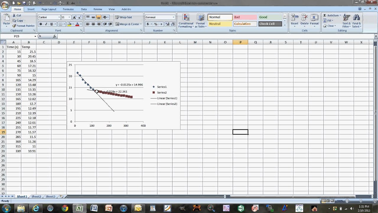
In the Analysis Tools box click Random Number Generation and then click OK. Click on Start select Programs select Microsoft Excel Or Click Microsoft Excel icon on computers desktop 2. Using Excel Heating and Cooling Curve 1.

Calculate the mean and average of the exam scores. The S Curve is a curve which is included in two different charts in Microsoft Excel. To create the ROC curve well highlight every value in the range F3G14.

Choose Column as the chart type and click Next. Now you can carry out the formatting of the chart. To present your data in a scatter chart or a line chart in Excel you can refer to this article.

Choose either Above Chart or Centered Overlay to set the position of your chart title. Now select all the generated points and go to the Insert tab in the Menu bar. They show how the temperature changes as a substance is cooled down.

We need to do these steps. Once both the cell ranges are selected go to the insert option. This value can be calculated using Mean 3 Standard Deviation 65-310.

Review graph and click Next. In the Number of Variables box type 1. In the cells of column A input the time in column B input cooling temperatures and in column C input heating temperatures 3.

Now to understand bell curve you need to know about two metrics. If you already know how to create a basic X-Y plot on Excel then skip ahead to page 3 and the section called Changing the Plot Appearance. There are a few differences to add best fit line or curve and equation between Excel 20072010 and 2013.

Now select XY Scatter Chart Category on the left side. Select Chart Title. Click on the third style Scatter with Smooth Lines.

Assume a student got a. So to Create an S Curve chart Select the cumulative work progress from week 1 to week 8 simultaneously by pressing the CTRL key to select the cells from week 1 to week 8. From the drop-down options select either the Scatter with smooth lines and.

Click the Fill Line category and. If you already know how to create a basic X-Y plot on Excel then skip ahead to page 3 and the section called Changing the Plot Appearance. Under that select a line with markers option chart.

First lets create a fake dataset to work with. Normal distribution will get populated for all the elements in the data. Next lets create a scatterplot to visualize the dataset.

The temperature of a pure substance changes only when there is no change of state. To edit this to a curved line right-click the data series and then select the Format Data Series button from the pop-up menu. I dont remember where I first found a way of doing this in Excel possibly the Carbon Trust but Ive had a MAC curve spreadsheet in my arsenal for some time now.

But to get a normal distribution curve Bell Curve follow the below steps. In the Insert tab click on the Scatter plot button a drop-down will appear. First click on All Charts.

Simple X-Y Plots Table 1 includes measured data on the current-voltage relationship of a diode that we can use for demonstration of the plotting and curve-fitting features of Excel. You can do this quickly by using the autofill option or use the fill handle and. I would like to create a MACC in excel 2007 the parameters are as follows.

Mean the average value of all the data points Standard Deviation its how different the data is from the mean value lets say you have 100 records with the mean is 50 but there is one value that is 10 the standard deviation is going to measure that. Select and highlight the range A1F2 and then click Insert Line or Area Chart Line. Open Add Chart Elements.

We apply the well-known average A2A11 and STDEVP A2A11 in excel for the values. On the Tools menu click Data Analysis. You can see the built-in styles at the top of the dialog box.

The annoying thing was setting it up to handle varying. Abatement options whereby the column AREA represents the savings madecost of implementation ie height is cost x width is saving. Create the ROC Curve.

Select the new added scatter chart and then click the Trendline More Trendline Options on the Layout tab. Simple X-Y Plots Table 1 includes measured data on the current-voltage relationship of a diode that we can use for demonstration of the plotting and curve-fitting features of Excel. Then well click the Insert tab along the top ribbon and then click Insert ScatterX Y to create the following plot.

Since there is no way of changing the width of each column in an Excel column chart we have to try something else. Cooling curves are the opposite. Navigate to the Design tab.

Here are the steps to create a bell curve for this dataset. Do not include column titlesheadings. See above screen shot.

Click once on your linear calibration curve chart. Fortunately this is fairly easy to do using the Trendline function in Excel. Select the original experiment data in Excel and then click the Scatter Scatter on the Insert tab.

The line graph is inserted with straight lines corresponding to each data point. Understand the cooling curve of substances and the way to score full marks in answering questions by watching the video in Mandarinhttpmrsaimunblogspot. To generate the random data that will form the basis for the bell curve follow these steps.

Ensure date of onset is in column before to the left of number of cases. The thermal energy released without a change in temperature is called Latent Heat. Cooling Curves Heating curves show how the temperature changes as a substance is heated up.

They are Scatter Chart and Line Chart. This tutorial provides a step-by-step example of how to fit an equation to a curve in Excel.

Freezing Point Depression Excel Demo Youtube

How To Graph Heating And Cooling Curves In Excel Youtube

How To Graph Heating And Cooling Curves In Excel Youtube

Pin On Excel